Design Principles of Fluid¶

Introduction¶

This document mainly introduces the underlying design principles Fluid to help users better understand the operation process of the framework.

After reading this document, you will learn about:

• internal execution process of Fluid

• How does Program express the model

• How does Executor perform operations

1. internal execution process of Fluid¶

Fluid uses a compiler-like execution process, which is divided into compile-time and runtime. Specifically, it includes : compiler defines Program, and an Executor is created to run the Program.

The flow chart of executing a local training task is as follows:

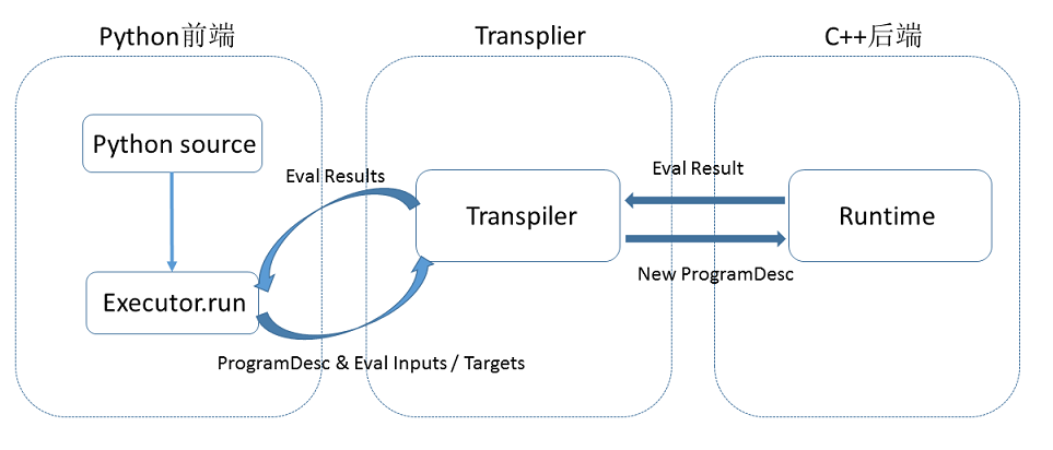
1. At compile time, the user writes a python program that adds variables (Tensor) and operations on variables (Operators or Layers) to a Program by calling the operators provided by Fluid. Users only need to describe the core forward calculations, and do not need to care about backward computing, distributed computing, and calculations on heterogeneous devices.

2. The original Program is converted to an intermediate descriptive language ProgramDesc within the platform:

3. The most important functional modules at compile time is Transpiler . Transpiler accepts a segment of ProgramDesc and outputs a segment of transformed ProgramDesc as the Program to be executed ultimately by backend Executor .

4. The backend Executor accepts the Program output from Transpiler , and executes the Operators in the Program in sequence (which can be analogized to the instructions in the programming language). During the execution, the Executor creates the required input and output for the Operator and manages them.

2. Design Principles of Program¶

After completing the network definition, there are usually 2 Programs in a Fluid program:

1. fluid.default_startup_program : defines various operations such as creating model parameters, input and output, and initialization of learnable parameters in the model.

default_startup_program can be automatically generated by the framework and can be used without visible manual creation. 

If the call changes the default initialization method of the parameter, the framework will automatically add the relevant changes to the default_startup_program

1. fluid.default_main_program : defines the neural network model, forward and backward calculations, and updates to the learnable parameters of the network by the optimization algorithm.

The core of using Fluid is to build ``default_main_program``

int main(){ //block 0
    int i = 0;
    if (i<10){ //block 1
        for (int j=0;j<10;j++){ //block 2
        }
    }
    return 0;
}

import paddle.fluid as fluid # block 0

limit = fluid.layers.fill_constant_batch_size_like(
	Input=label, dtype='int64', shape=[1], value=5.0)
cond = fluid.layers.less_than(x=label, y=limit)

ie = fluid.layers.IfElse(cond)
with ie.true_block(): # block 1
	true_image = ie.input(image)
	hidden = fluid.layers.fc(input=true_image, size=100, act='tanh')
	prob = fluid.layers.fc(input=hidden, size=10, act='softmax')
	ie.output(prob)

with ie.false_block(): # block 2
	false_image = ie.input(image)
	hidden = fluid.layers.fc(
		input=false_image, size=200, act='tanh')
	prob = fluid.layers.fc(input=hidden, size=10, act='softmax')
	ie.output(prob)

prob = ie()

 message BlockDesc {
  required int32 parent = 1;
  repeated VarDesc vars = 2;
  repeated OpDesc ops = 3;
}

message ProgramDesc {
  repeated BlockDesc blocks = 1;
}

message OpDesc {
  AttrDesc attrs = 1;
  ...
}

message AttrDesc {
  required string name = 1;

  enum AttrType {
	INT = 1,
	STRING = 2,
	...
	BLOCK = ...
  }
  required AttrType type = 2;

  optional int32 block = 10; // when type == BLOCK
  ...
}

3. Design Principles of Executor¶

Executor will accept a ProgramDesc, a block_id and a Scope at runtime. ProgramDesc is a list of block, each containing all the parameters in block and the protobuf definition of operator; block_id specifying the entry block; Scope is the container for all variable instances.

The specific process of compilation and execution is shown in the following figure:

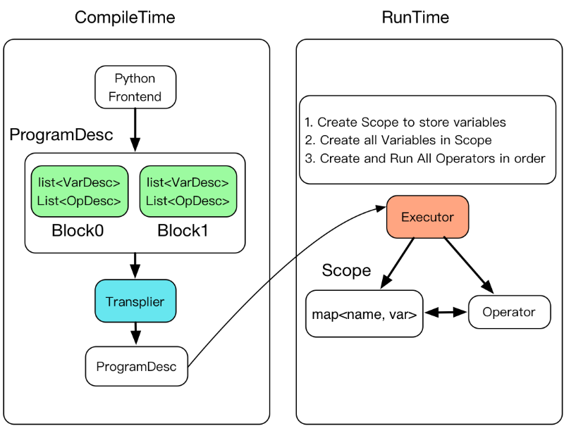
1. Executor creates a Scope for each block. Block is nestable, so Scope is nestable

2. Create all variables in Scope

3. Create and Run all operators in order

C++ implementation code of Executor is as follows:

class Executor{
		public:
			void Run(const ProgramDesc& pdesc,
							scope* scope,
							int block_id) {
						auto& block = pdesc.Block(block_id);

						// Create all variables
						for (auto& var : block.AllVars())
								scope->Var(Var->Name());
						}

						// Create OP and execute in order
						for (auto& op_desc : block.AllOps()){
								auto op = CreateOp(*op_desc);
								op->Run(*local_scope, place_);
						}
			}
	};

Create Executor

Fluid uses Fluid.Executor(place) to create an Executor. The place attribute is defined by user and represents where the program will be run.

The following code example creates an Executor that runs on CPU:

cpu=fluid.CPUPlace()
exe = fluid.Executor(cpu)

Run Executor

Fluid uses Executor.run to run the program. In the definition, the data is obtained through the Feed dict, and the result is obtained through fetch_list:

...
x = numpy.random.random(size=(10, 1)).astype('float32')
outs = exe.run(
		feed={'X': x},
		fetch_list=[loss.name])

Code Instance¶

This section introduces how the above is implemented in your code through a simple linear regression example in the Fluid Programming Guide.

Define Program

You can freely define your own data and network structure, which will be received as a Program by Fluid. The basic structure of Program is some blocks. The Program in this section contains only block 0:

#Load function library
import paddle.fluid as fluid #block 0
import numpy

# Define data
train_data=numpy.array([[1.0],[2.0],[3.0],[4.0]]).astype('float32')
y_true = numpy.array([[2.0],[4.0],[6.0],[8.0]]).astype('float32')
# Define the network
x = fluid.layers.data(name="x",shape=[1],dtype='float32')
y = fluid.layers.data(name="y",shape=[1],dtype='float32')
y_predict = fluid.layers.fc(input=x,size=1,act=None)
#definition loss function
cost = fluid.layers.square_error_cost(input=y_predict,label=y)
avg_cost = fluid.layers.mean(cost)
#defined optimization method
sgd_optimizer = fluid.optimizer.SGD(learning_rate=0.01)
sgd_optimizer.minimize(avg_cost)

Finishing the above definition is at the same time finishing the construction process of fluid.default_main_program. fluid.default_main_program carries the neural network model, forward and backward calculation, and the optimization algorithm which updates the learnable parameters in the network.

At this point you can output this Program to observe the defined network:

print(fluid.default_main_program().to_string(True))

The complete ProgramDesc can be viewed locally. The first three variables are excerpted and displayed as follows:

blocks {
  idx: 0
  parent_idx: -1
  vars {
	name: "mean_1.tmp_0"
	type {
	  type: LOD_TENSOR
	  lod_tensor {
		tensor {
		  data_type: FP32
		  dims: 1
		}
	  }
	}
	persistable: false
  }
  vars {
	name: "square_error_cost_1.tmp_1"
	type {
	  type: LOD_TENSOR
	  lod_tensor {
		tensor {
		  data_type: FP32
		  dims: -1
		  dims: 1
		}
		lod_level: 0
	  }
	}
	persistable: false
  }
  vars {
	name: "square_error_cost_1.tmp_0"
	type {
	  type: LOD_TENSOR
	  lod_tensor {
 		tensor {
		data_type: FP32
		  dims: -1
		  dims: 1
		}
		lod_level: 0
	  }
	}
	persistable: false
	...

As you can see from the output, the entire definition process is transformed into a ProgramDesc inside the framework, indexed by block idx. There is only one block in this linear regression model, and ProgramDesc has only one piece of BlockDesc, namely Block 0.

BlockDesc contains defined vars and a series of ops. Take input x as an example. In python code, x is 1D data of data type “float 32”:

x = fluid.layers.data(name="x",shape=[1],dtype='float32')

In BlockDesc, the variable x is described as:

vars {
	name: "x"
	type {
	  type: LOD_TENSOR
	  lod_tensor {
		tensor {
		  data_type: FP32
		  dims: -1
		  dims: 1
		}
		lod_level: 0
	  }
	}
	persistable: false

All data in Fluid are LoD-Tensor, and for data without sequence information (such as variable X here), lod_level=0.

dims represents the dimension of the data, and in the example x has the dimension of [-1,1], where -1 is the dimension of the batch. When the specific value cannot be determined, Fluid automatically uses the -1 as placeholder.

The parameter persistable indicates whether the variable is a persistent variable throughout the training process.

Create Executor

Fluid uses Executor to perform network training. For details on Executor operation, please refer to [Executor Design Principles](#Executor Design Ideas). As a user, there is actually no need to understand the internal mechanism.

To create an Executor, simply call fluid.Executor(place). Before that, please define a place variable based on the training site:

 #Execute training on CPU
 cpu = fluid.CPUPlace()
 #Create Executor
 exe = fluid.Executor(cpu)

Run Executor

Fluid uses Executor.run to run a program.

Before the network training is actually performed, parameter initialization must be performed first. Among them, default_startup_program defines various operations such as creating model parameters, input and output, and initialization of learnable parameters in the model.

 #Parameter initialization
 exe.run(fluid.default_startup_program())

Since there are multiple columns of incoming and outgoing data, fluid defines transferred data through the feed mapping, and fetch_list takes out the expected result:

# Start training
 outs = exe.run(
 	 feed={'x':train_data,'y':y_true},
	 fetch_list=[y_predict.name,avg_cost.name])

The above code defines that train_data is to be passed into the x variable, y_true is to be passed into the y variable, and output the predicted value of y and the last round value of cost.

The output is:

[array([[1.5248038],
	   [3.0496075],
	   [4.5744114],
	   [6.099215 ]], dtype=float32), array([1.6935859], dtype=float32)]

Till now you have already be notified of the core concepts of the internal execution process of Fluid. For more details on the usage of the framework, please refer to the User Guide related content, Model Library also provides you with a wealth of model examples for reference.